MDM4U Unit 4:
Probability Distributions
4-1 Probability Distributions
Learning Goal:
I can ...
- explain and apply my understanding of a probability distribution
Lesson:
Read and take notes as necessary:
1) Introduction to Distributions
In Unit 3, you looked at the probability of individual outcomes. This unit focuses on models that show the probabilities of all possible outcomes of an experiment. Distribution models have applications in many fields including science, game theory, economics, telecommunications, and manufacturing.
Many probability experiments have numerical outcomes (outcomes that can be counted or measured).
A random variable, X, has a single value (x) for each outcome in an experiment.
Random variables can be discrete or continuous.
The probability of a random variable having a particular value x is represented as P(X = x), or P(x) for short.
2) Examples of Probability Distributions
Example 1:
1) Introduction to Distributions
In Unit 3, you looked at the probability of individual outcomes. This unit focuses on models that show the probabilities of all possible outcomes of an experiment. Distribution models have applications in many fields including science, game theory, economics, telecommunications, and manufacturing.
Many probability experiments have numerical outcomes (outcomes that can be counted or measured).
A random variable, X, has a single value (x) for each outcome in an experiment.
- For example, if X is the number rolled with a die, then x could have a value of 1, 2, 3, 4, 5, or 6.
Random variables can be discrete or continuous.
- Discrete variables can only take on a finite set of integer values (e.g. the number rolled with a die can only be 1, 2, 3, 4, 5, or 6).
- Continuous variables have an infinite number of possible values within an interval (e.g. the time it takes to drive to Toronto can range anywhere from an hour to several hours, with an infinite number of possibilities in between).
The probability of a random variable having a particular value x is represented as P(X = x), or P(x) for short.
2) Examples of Probability Distributions
Example 1:
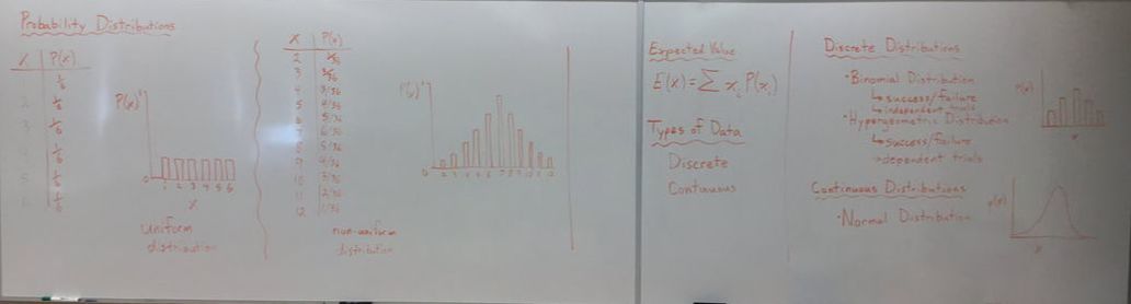
- We can create the following probability distribution table for the outcomes of rolling a single six-sided die:
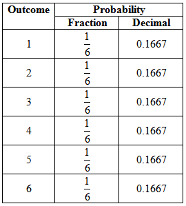
- This is an example of a uniform probability distribution (all outcomes are equally likely).
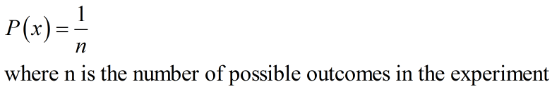
- To calculate the probability in a discrete uniform distribution:
Example 2:
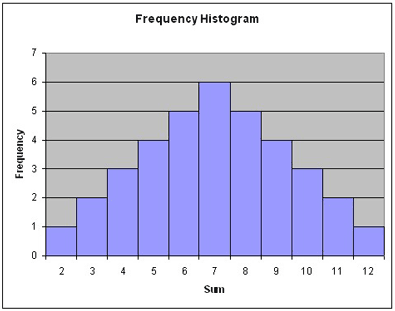
- Using Counting Principles, we can create the following probability distribution table for the sum obtained by rolling two six-sided dice:
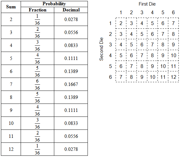
- This is not a uniform probability distribution, as not all of the outcomes are equally as likely to occur.
- A frequency histogram shows how often each value in the distribution occurs. The independent variable is the random variable while the dependent variable is frequency.
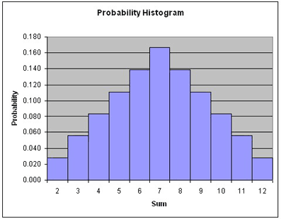
- A probability histogram shows the same information except that the dependent variable is probability instead of frequency.
|
|
3) Expected Value for Discrete Probability Distribution
As with all probability distributions, predictions can be made.
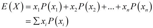
The expected value of a probability distribution is the predicted average of all possible outcomes and is denoted by the notation E(X).
To calculate the expected value, find the sum of all values multiplied by the probability of each value occurring.
3) Example of Expected Value
What is the expected value when you roll two six-sided dice? You can figure this out using the probability distribution table above.
What is the expected value when you roll two six-sided dice? You can figure this out using the probability distribution table above.
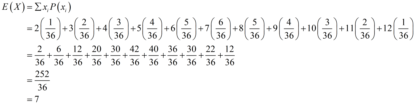
- That means that when you roll two six-sided dice, the expected outcome is a sum of 7.
You can use expected value to determine if a game is fair. The expected value in a fair game is 0 (see the examples in the videos below).
4) Applying Probability Distributions
Practice:
1) Complete the following textbook questions:
- Page 374, # 1 - 6, 8 - 12, 17, 19
4-2 Binomial Distributions
Learning Goal:
I can ...
- identify the appropriate time to use and successfully apply binomial distributions
Lesson:
Read and take notes as necessary:
1) Binomial Distributions
A binomial distribution is a probability distribution in which each trial can be thought of in terms of either "success" or "failure". If there are 2 possible outcomes for any given trial, these are called Bernoulli Trials. For example:
If the probability of an event being a success is p, and the probability of an event being a failure is q, then:
For such binomial distributions:
2) Probability and Expected Value in a Binomial Distribution
For a binomial distribution, you can calculate the probability of x successes in n Bernoulli trials using this formula:
1) Binomial Distributions
A binomial distribution is a probability distribution in which each trial can be thought of in terms of either "success" or "failure". If there are 2 possible outcomes for any given trial, these are called Bernoulli Trials. For example:
- A manufacturing company needs to know the expected number of defective units among its products. "Success" means the products are not defective, and "Failure" means the products are defective.
- A polling company wants to estimate how many people are in favour of a new law. "Success" is a person who supports the new law, and "Failure" is a person who does not support the new law.
If the probability of an event being a success is p, and the probability of an event being a failure is q, then:
- p + q = 1
- q = 1 - p
For such binomial distributions:
- all trials have only two possible outcomes (success or failure)
- all trials are independent
- the probability of success is the same in every trial (the outcome of one trial does not affect the probabilities of any of the later trials)
- the random variable X is the number of successes in a set number of Bernoulli trials
2) Probability and Expected Value in a Binomial Distribution
For a binomial distribution, you can calculate the probability of x successes in n Bernoulli trials using this formula:
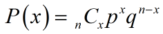
where n is the number of Bernoulli trials, p is the probability of success on any individual trial, and q = 1 - p is the probability of failure.
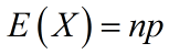
Since the probability for all trials is the same, the expectation for a success in any one trial is p.
The expected number of successes in n independent trials is:
Since the probability for all trials is the same, the expectation for a success in any one trial is p.
The expected number of successes in n independent trials is:
3) Examples for Binomial Distributions
Work:
4-3 Hypergeometric Distributions
Learning Goal:
I can ...
- identify the appropriate time to use and successfully apply hypergeometric distributions
Lesson:
Read and take notes as necessary:
1) Hypergeometric Distributions
A hypergeometric distribution is similar to a binomial distribution in that it has two possible outcomes: success or failure.
However, while the binomial distribution relies on independent trials, the hypergeometric distribution relies on dependent trials. The probability of success changes with each successive trial.
For such hypergeometric distributions:
2) Probability and Expected Value in a Hypergeometric Distribution
To calculate the probability of x successes in r dependent trials, use this formula:
1) Hypergeometric Distributions
A hypergeometric distribution is similar to a binomial distribution in that it has two possible outcomes: success or failure.
However, while the binomial distribution relies on independent trials, the hypergeometric distribution relies on dependent trials. The probability of success changes with each successive trial.
For such hypergeometric distributions:
- all trials have only two possible outcomes (success or failure)
- all trials are dependent (the probability of success changes as each trial is made.
- the random variable X is the number of successes in a set number of Bernoulli trials
2) Probability and Expected Value in a Hypergeometric Distribution
To calculate the probability of x successes in r dependent trials, use this formula:
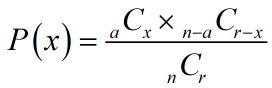
where a is the number of successful outcomes among a total of n possible outcomes, and r is the number of dependent trials.
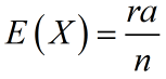
The expected number of successes in n dependent trials is:
The expected number of successes in n dependent trials is:
3) Examples for Hypergeometric Distributions
Practice:
4-4 Continuous Probability Distributions
Learning Goal:
I can ...
- identify the appropriate time to use and successfully apply continuous probability distributions
Lesson:
Watch and take notes as necessary.
Practice:
4-5 Normal Distributions
Learning Goal:
I can ...
- identify the appropriate time to use and successfully apply normal distributions
Lesson:
Read and take notes as necessary:
1) Characteristics of the Normal Distribution
The Normal Distribution ...
1) Characteristics of the Normal Distribution
The Normal Distribution ...
- is a continuous distribution (not discrete)
- is symmetrical across the mean
- has the shape of a bell (a bell curve)
- never touches the x-axis

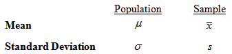
Remember:
- Mean is the average
- Standard Deviation is a measure of how spread out the data are
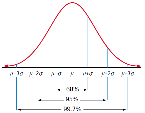
In a Normal Distribution:
- Approximately 68% of the data are within one standard deviation of the mean
- Approximately 95% of the data are within two standard deviations of the mean
- Approximately 99.7% of the data are within three standard deviations of the mean
2) Probability in a Normal Distribution
Probability of a continuous distribution is the area under the curve.
For a Normal Distribution the total area under the curve is 1 (or 100% probability)
A z-Score Table can be used to determine the area under just part of a normal distribution curve.
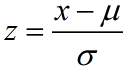
Remember how to calculate a z-score:
Probability of a continuous distribution is the area under the curve.
For a Normal Distribution the total area under the curve is 1 (or 100% probability)
A z-Score Table can be used to determine the area under just part of a normal distribution curve.
- If the z-score is negative, the value is less than the mean (left side)
- If the z-score is positive, the value is more than the mean (right side)
Remember how to calculate a z-score:
3) Probability for a Normal Distribution Example
Practice:
4-6 Normal Models of Discrete Distributions
Learning Goal:
I can ...
- model discrete data with a normal distribution
- solve related problems
Lesson:
Read and take notes as necessary:
1) Remember ...
Random variables can be discrete or continuous.
2) Normal Models for Discrete Data
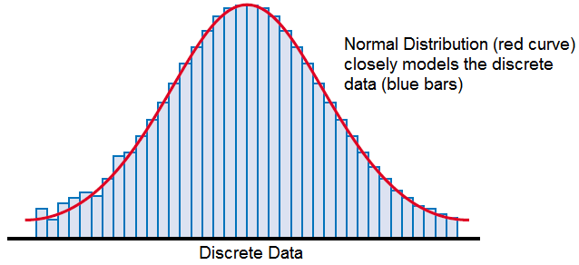
All the examples of normal distributions you have seen so far have modelled continuous data.
However, there are many situations where discrete data can also be modelled as normal distributions. If the data set is reasonably large, and the data fall into a symmetric bell shape, it makes sense to try fitting a smooth normal curve to them.
1) Remember ...
Random variables can be discrete or continuous.
- Discrete variables can only take on a finite set of integer values (e.g. the number rolled with a die can only be 1, 2, 3, 4, 5, or 6).
- Continuous variables have an infinite number of possible values within an interval (e.g. the time it takes to drive to Toronto can range anywhere from an hour to several hours, with an infinite number of possibilities in between).
2) Normal Models for Discrete Data
All the examples of normal distributions you have seen so far have modelled continuous data.
However, there are many situations where discrete data can also be modelled as normal distributions. If the data set is reasonably large, and the data fall into a symmetric bell shape, it makes sense to try fitting a smooth normal curve to them.
For a continuous distribution, the probabilities are for ranges of values.
This means that when a normal distribution is being used to model discrete data, discrete values have to be treated as though they were continuous. Instead of looking for a single value, you need to change it into a range of values.
3) Example of Normal Models for Discrete Data
- For example, all probabilities listed on the Z-Score Table are of the form P(Z < z) not P(Z = z).
This means that when a normal distribution is being used to model discrete data, discrete values have to be treated as though they were continuous. Instead of looking for a single value, you need to change it into a range of values.
- For example, let X be the number of boys in a class;
- the probability of having 12 boys in a class is not P(X = 12), but rather P(11.5 < X < 12.5)
3) Example of Normal Models for Discrete Data
4) Normal Approximation of the Binomial Distribution
Remember ...
- The binomial distribution is a discrete probability distribution with n Bernoulli trials (either success or failure)
- p is the probability of success
- q = 1 - p is the probability of failure
The normal distribution is a very good approximation of the binomial distribution as long as two conditions are met:
- np > 5
- nq > 5
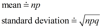
Since the normal distribution requires the mean and standard deviation values to perform the calculations, the binomial distribution must have some way of approximating these values. For a binomial distribution:
5) Example of Normal Approximation of the Binomial Distribution
Practice:
1) Complete the following questions: 2) Check your answers.